Note: This post is easier to follow if you know a bit of calculus. I've still included some proofs for the sake of explanation, so feel free to skip the parts you already know.

Right angles and rectangles always feel comfortable to us. Humanity invented the Cartesian coordinate system. And most computer monitors have pixels arranged in a grid of hundreds to thousands of pixels across and down, which you can address with Cartesian coordinates. I suppose it's because drawing the screen on a Cartesian grid makes it easiest and most flexible to manage each individual pixel.

Suppose someone is developing a game with an engine that only provides the four basic arithmetic operations. There's some shape drawn on a Cartesian plane, and they need to rotate it. How would they do it?

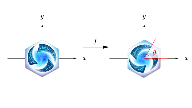
Actually, math already knows the answer. For a pixel at coordinates $\left ( x, y\right )$, the rotated coordinates $\left ( x′, y′\right )$ are

in other words,

which is self-evident. Do this once for the $\left ( x, y\right )$ of every pixel in the original image, and you get the rotated image. Easy, right?

You want me to compute trig functions with nothing but the four basic operations?

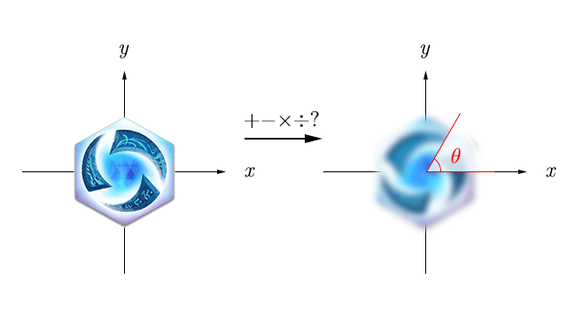
Since we're discussing how computers calculate trigonometric functions, we should only use operations a computer can do. On a processor that supports only very basic operations, that is.

So how on earth can we approximate trigonometric functions? Once we have $\sin$ and $\cos$, we can get $\tan$ and the like by division, so let's focus on finding $\sin$ and $\cos$.

Couldn't we just approximate trig functions with polynomials?

Polynomials can be computed with just the four basic operations, so we could build a polynomial that looks like the graph of a trig function and plug values into that!

But how do we actually find that polynomial? This is where the Taylor series comes in.

Taylor Series

With the Taylor series, you can approximate any differentiable function with a polynomial. Does such black magic really exist? Yes, amazingly, it does!

Proof

First, let's take the definite integral of some function $f^\prime\left(x\right )$ from $a$ to $x$. By the definition of calculus, it can be written as follows.

Now let's rearrange the equation above.

Now let's integrate $-1$ and differentiate $-f^\prime\left(t\right )$ to apply integration by parts. If $f\left(x\right )$ is infinitely differentiable, we can apply integration by parts infinitely many times too. So

Here, $x$, which doesn't depend on the variable of integration $t$, is treated as a constant. Expanding this equation gives

Finally, moving $f\left ( a \right )$ to the other side gives

That is, if $f^{\left( n \right)}$ is the function obtained by differentiating $f$ $n$ times,

is derived. This approximation works for any value you put in for $a$.

So what does this have to do with trig functions!

Trigonometric functions are infinitely differentiable. So if we put a trig function in place of $f$, we can approximate the trig function with a polynomial. For a trig function $f\left ( x \right )$, substituting $0$ for $a$ gives

and letting $f\left ( x \right ) = \sin x$ and substituting,

Simplifying,

Likewise,

Compared to the steps in between, it turned into a really simple formula. What's more, we've achieved our ultimate goal of expressing trig functions with only the four basic operations! (Factorials are just repeated multiplication, after all!)

But the formula is, well… infinite. What should we do about that? We all know that floating-point variables aren't all that accurate anyway. So we can compute the formula up to a certain point and just ignore the error beyond that.

Let's compute the polynomial we found above only up to the term of degree $n$ and ignore the rest. Let's call this the degree-$n$ approximation. From here on, I'll raise the degree step by step and plot the graph of the degree-$n$ approximation.

Graphs

▶ Degree-1 approximation: $f\left ( x \right ) = x$

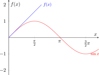
… Doesn't look similar at all. Next!

▶ Degree-3 approximation: $f\left ( x \right ) = x-\dfrac{x^3}{3!}$

It seems to have gotten the hang of it near the start, but it starts getting a little off before even reaching $\dfrac{\pi}{2}$, and then it nosedives. Next!

▶ Degree-5 approximation: $f\left ( x \right ) = x-\dfrac{x^3}{3!} + \dfrac{x^5}{5!}$

Now it's similar at $\dfrac{\pi}{2}$ too! Next!

▶ Degree-7 approximation: $f\left ( x \right ) = x-\dfrac{x^3}{3!} + \dfrac{x^5}{5!}- \dfrac{x^7}{7!}$

It's pretty close even around $pi$ now. Let's do a few more.

▶ Degree-9 approximation: $f\left ( x \right ) = x-\dfrac{x^3}{3!} + \dfrac{x^5}{5!}-\dfrac{x^7}{7!} + \dfrac{x^9}{9!}$

It's almost identical to the original function. Honestly, from here on, it looks like you could just use it as is for $0 < x < \pi$ without much error. Since $sin$ is periodic and symmetric anyway, as long as it's accurate on $0 < x < \dfrac{\pi}{2}$, you can compute other ranges using the properties of the function.

▶ Degree-11 approximation: $f\left ( x \right ) = x-\dfrac{x^3}{3!} + \dfrac{x^5}{5!}- \dfrac{x^7}{7!} + \dfrac{x^9}{9!}- \dfrac{x^{11}}{11!}$

It's getting hard to tell how much they differ just by looking. Let me plot just one last one, the degree-13 approximation.

▶ Degree-13 approximation: $f\left ( x \right ) = x- \dfrac{x^3}{3!} + \dfrac{x^5}{5!}- \dfrac{x^7}{7!} + \dfrac{x^9}{9!}- \dfrac{x^{11}}{11!} + \dfrac{x^{13}}{13!}$

Within the range of the graph, the curves are practically identical.

Implementations in Programming Languages

The native code of OpenJDK's StrictMath implements trig functions using a degree-13 approximation. For accuracy, it doesn't use the degree-13 approximation as is, but modifies it slightly like this.

So when $r$ is defined like this,

$\sin x$ can be expressed like this.

Let's look at an example. When the sin function calls __kernel_sin, if $|x| \prec \pi/4$ in the code, the values of y and iy are both 0. For other ranges, it shifts the input into an appropriate range and computes the value of __kernel_sin or __kernel_cos.

#include "fdlibm.h"
#ifdef __STDC__
    static const double
#else
    static double
#endif
half = 5.00000000000000000000e-01, /* 0x3FE00000, 0x00000000 */
S1 = -1.66666666666666324348e-01, /* 0xBFC55555, 0x55555549 */
S2 = 8.33333333332248946124e-03, /* 0x3F811111, 0x1110F8A6 */
S3 = -1.98412698298579493134e-04, /* 0xBF2A01A0, 0x19C161D5 */
S4 = 2.75573137070700676789e-06, /* 0x3EC71DE3, 0x57B1FE7D */
S5 = -2.50507602534068634195e-08, /* 0xBE5AE5E6, 0x8A2B9CEB */
S6 = 1.58969099521155010221e-10; /* 0x3DE5D93A, 0x5ACFD57C */

#ifdef __STDC__
    double __kernel_sin(double x, double y, int iy)
#else
    double __kernel_sin(x, y, iy) double x,y; int iy; /* iy=0 if y is zero */
#endif
{
    double z,r,v; int ix;
    ix = __HI(x)&0x7fffffff; /* high word of x */
    if(ix < 0x3e400000) /* |x| < 2**-27 */ {
        if((int)x==0) return x;
    } /* generate inexact */
    z = x*x;
    v = z*x;
    r = S2+z*(S3+z*(S4+z*(S5+z*S6)));
    if(iy==0) return x+v*(S1+z*r);
    else return x-((z*(half*y-v*r)-y)-v*S1);
}

In the source, you can see that the coefficients of the approximation are approximated and hardcoded as
$S1 = -\dfrac{1}{3!} \approx -1.66666667 \times {10}^{-1}$
$S2 = \dfrac{1}{5!} \approx 8.33333333 \times {10}^{-2}$
$S3 = -\dfrac{1}{7!} \approx -1.98412698 \times {10}^{-4}$
$S4 = \dfrac{1}{9!} \approx 2.75573137 \times {10}^{-6}$
$S5 = -\dfrac{1}{11!} \approx -2.50521084 \times {10}^{-8}$
$S6 = \dfrac{1}{13!} \approx 1.58969099 \times {10}^{-10}$
. It also computes $z=x^2$ and $v=zx=x^3$. If you used the degree-13 approximation as is, you'd need 1, 3, 5, …, 13 multiplications for each term, but treating $x^2$ as a new constant cuts down on multiplications, which I think is probably why they used this approach.

Are there other ways to calculate them?

Of course there are. For example, you can also approximate trig function values using the CORDIC (COordinate Rotation DIgital Computer) algorithm, devised by Volder in 1956.

To explain it briefly: at the very top, I introduced the matrix we multiply by to rotate as

but the CORDIC algorithm expresses this using only the $\tan$ function, transforming it into

and, so that computers can calculate it quickly, hardcodes the values of $\gamma_i$ such that $\tan \left(\gamma_i\right) = \pm2^{-i}$, i.e. $\arctan\left(2^{-i}\right)$, along with the corresponding values of $\dfrac{1}{\sqrt{1 + \tan^2 \left(\gamma_i\right)}}$. Then, increasing $i$ one by one until it gets close to the desired angle, it carries out the matrix computation while
adding or subtracting $\arctan\left(2^{-i}\right)$.

This algorithm is mainly used in calculators, and it has also been used in Intel's 8087 through 80486 CPUs.

And that's how computers calculate trigonometric functions.